This project encompassed both collaborative and individual components. As a team, we developed a product concept and identified a dataset relevant to our idea. The task involved pitching our application, designed specifically for students, focusing on finance, innovation, and enterprise. Our pitch was presented as a video, which I’ve embedded on the first page of the PDF above containing my individual report.

Individually, we were responsible for diving deeper into the technical side of our pitch. This included conducting data analysis, identifying the market gap, understanding target customers, and outlining a strategic approach to product sales. While teamwork was encouraged, each member was expected to make a unique and meaningful contribution in their final report.

Below are key snippets of code I developed during the data analysis phase, which played a critical role in shaping our product’s direction. I led this part of the project, as it closely aligned with my strengths. Using a preliminary dataset, I informed our pricing strategy, while an Uber Analysis Dataset enabled me to identify market gaps and opportunities. Below, I’ve included snippets from the latter dataset to demonstrate its role in our decision-making process.

Importing Data and Intial Analysis

Importing librarys

import matplotlib.pyplot as plt
import pandas as pd
import plotly.express as px
import seaborn as sns

Importing dataset

df = pd.read_csv("UberDataset.csv")
df.head()

	START_DATE	END_DATE	CATEGORY	START	STOP	MILES	PURPOSE
0	01/01/2016 21:11	01/01/2016 21:17	Business	Fort Pierce	Fort Pierce	5.1	Meal/Entertain
1	01/02/2016 01:25	01/02/2016 01:37	Business	Fort Pierce	Fort Pierce	5.0	NaN
2	01/02/2016 20:25	01/02/2016 20:38	Business	Fort Pierce	Fort Pierce	4.8	Errand/Supplies
3	01/05/2016 17:31	01/05/2016 17:45	Business	Fort Pierce	Fort Pierce	4.7	Meeting
4	01/06/2016 14:42	01/06/2016 15:49	Business	Fort Pierce	West Palm Beach	63.7	Customer Visit

Looking at data types of columns

df.info()

<class 'pandas.core.frame.DataFrame'>
RangeIndex: 1155 entries, 0 to 1154
Data columns (total 7 columns):
 #   Column      Non-Null Count  Dtype  
---  ------      --------------  -----  
 0   START_DATE  1155 non-null   object 
 1   END_DATE    1155 non-null   object 
 2   CATEGORY    1155 non-null   object 
 3   START       1155 non-null   object 
 4   STOP        1155 non-null   object 
 5   MILES       1155 non-null   float64
 6   PURPOSE     653 non-null    object 
dtypes: float64(1), object(6)
memory usage: 63.3+ KB

Standardize column names to lowercase for consistency

df.columns = df.columns.str.lower()
df.head()

	start_date	end_date	category	start	stop	miles	purpose
0	01/01/2016 21:11	01/01/2016 21:17	Business	Fort Pierce	Fort Pierce	5.1	Meal/Entertain
1	01/02/2016 01:25	01/02/2016 01:37	Business	Fort Pierce	Fort Pierce	5.0	NaN
2	01/02/2016 20:25	01/02/2016 20:38	Business	Fort Pierce	Fort Pierce	4.8	Errand/Supplies
3	01/05/2016 17:31	01/05/2016 17:45	Business	Fort Pierce	Fort Pierce	4.7	Meeting
4	01/06/2016 14:42	01/06/2016 15:49	Business	Fort Pierce	West Palm Beach	63.7	Customer Visit

Checking for missing values in the dataset

df.isnull().sum()
#no missing values found

start_date      0
end_date        0
category        0
start           0
stop            0
miles           0
purpose       502
dtype: int64

Simple descriptive statistics of each numerical column

df.describe()

	miles
count	1155.000000
mean	10.566840
std	21.579106
min	0.500000
25%	2.900000
50%	6.000000
75%	10.400000
max	310.300000

Data Cleaning

Checked & removed duplicates

duplicated_data = df[df.duplicated()]
print(duplicated_data.shape)

df = df.drop_duplicates(keep='first')

(1, 7)

Encode categorical variables using one-hot encoding

data_encoded = pd.get_dummies(df, columns=['category', 'purpose'], drop_first=True)

Converted date columns into date time

df["start_date"] = pd.to_datetime(df["start_date"], errors="coerce")
df["end_date"] = pd.to_datetime(df["end_date"], errors="coerce")

Handling missing values

# Handle missing values by dropping rows with missing 'start' or 'stop' and filling 'purpose' with 'unknown'
df.dropna(subset=['start', 'stop'], inplace=True)
df['purpose'] = df['purpose'].fillna("Unknown")

Feature engineering, created new column for trip date

df["date"] = df["start_date"].dt.date

Ensured the dataset is sorted by date

df = df.sort_values('start_date')
df.set_index('start_date', inplace=True)

Analysis

Returns first few rows of dataset to check

df.head()

	end_date	category	start	stop	miles	purpose	date
start_date
2016-01-01 21:11:00	2016-01-01 21:17:00	Business	Fort Pierce	Fort Pierce	5.1	Meal/Entertain	2016-01-01
2016-01-02 01:25:00	2016-01-02 01:37:00	Business	Fort Pierce	Fort Pierce	5.0	Unknown	2016-01-02
2016-01-02 20:25:00	2016-01-02 20:38:00	Business	Fort Pierce	Fort Pierce	4.8	Errand/Supplies	2016-01-02
2016-01-05 17:31:00	2016-01-05 17:45:00	Business	Fort Pierce	Fort Pierce	4.7	Meeting	2016-01-05
2016-01-06 14:42:00	2016-01-06 15:49:00	Business	Fort Pierce	West Palm Beach	63.7	Customer Visit	2016-01-06

Plot trip frequency over time plot code

plt.figure(figsize=(11, 7))
sns.lineplot(x=df["date"].value_counts().sort_index().index,
             y=df["date"].value_counts().sort_index().values, marker="o")
plt.xlabel("date")
plt.ylabel("Number of Trips")
plt.title("Uber Trips Over Time")
plt.xticks(rotation=45)
plt.show()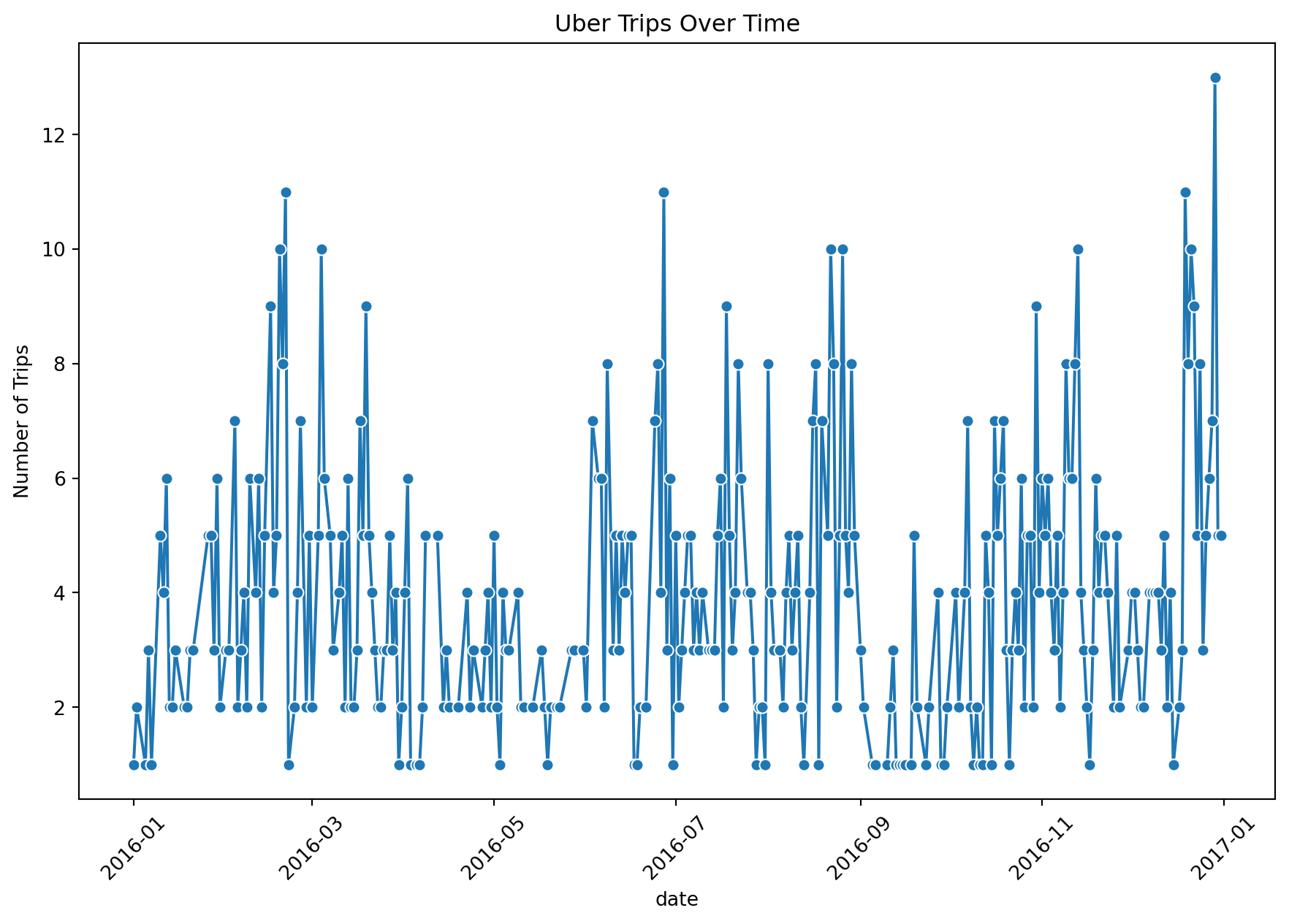

Top 10 most common pickup and drop-off locations plot code

top_pickups = df["start"].value_counts().head(10)
top_dropoffs = df["stop"].value_counts().head(10)

fig, axes = plt.subplots(1, 2, figsize=(9, 3))

sns.barplot(x=top_pickups.values, y=top_pickups.index, ax=axes[0], palette="Blues_r", hue=top_pickups.index, dodge=False)  
axes[0].set_title("Top 10 Pickup Locations")
axes[0].set_xlabel("Number of Trips")
axes[0].legend([],[], frameon=False)  
sns.barplot(x=top_dropoffs.values, y=top_dropoffs.index, ax=axes[1], palette="Greens_r", hue=top_dropoffs.index, dodge=False)
axes[1].set_title("Top 10 Drop-off Locations")
axes[1].set_xlabel("Number of Trips")
axes[1].legend([],[], frameon=False) 

plt.tight_layout()
plt.show()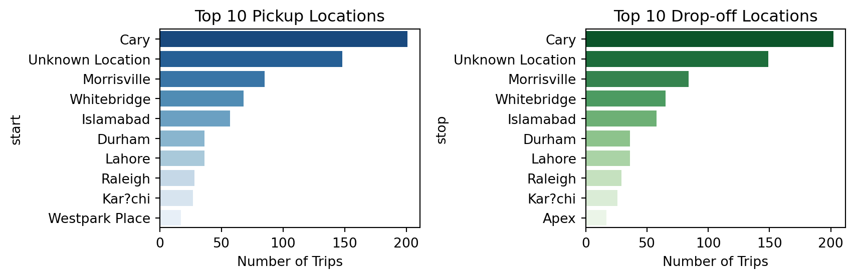

Code for plot of count of trips by purpose

trip_purpose_counts = df["purpose"].value_counts()
plt.figure(figsize=(9, 5))
sns.barplot(x=trip_purpose_counts.index, y=trip_purpose_counts.values, hue=trip_purpose_counts.index, palette="Oranges", legend=False) 
plt.xlabel("Purpose of Trip")
plt.ylabel("Number of Trips")
plt.title("Trip Purpose Distribution")
plt.xticks(rotation=45)
plt.show()

#Main purpose isn't known but second is a meeting which could be relative to commuting with commuting having little, below we see it has the highest average distance by purpose, which backs up our product in relation a student carpooling application which would aid in their commute.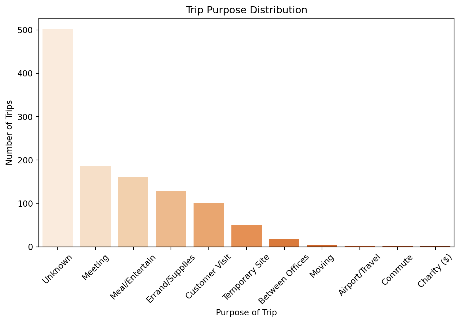

Code for plot of average trip distance by purpose

avg_miles_purpose = df.groupby("purpose")["miles"].mean().sort_values()
plt.figure(figsize=(9, 5))
sns.barplot(x=avg_miles_purpose.index, y=avg_miles_purpose.values, hue=avg_miles_purpose.index, dodge=False, palette="Blues", legend=False)  
plt.xlabel("Purpose of Trip")
plt.ylabel("Average Miles Traveled")
plt.title("Average Trip Distance by Purpose")
plt.xticks(rotation=45)
plt.show()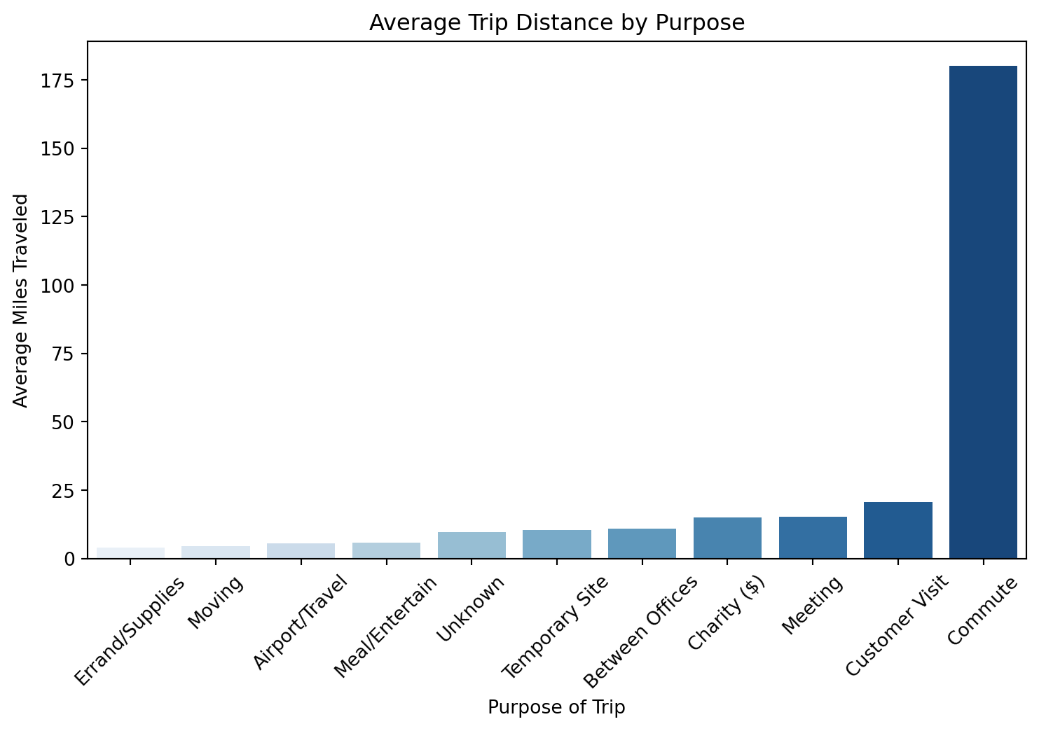

Plot for hourly trip analysis of the day

df["hour"] = df.index.hour
plt.figure(figsize=(9, 5))
sns.countplot(x=df["hour"], hue=df["hour"], dodge=False, palette="coolwarm", legend=False) 
plt.xlabel("Hour of the Day")
plt.ylabel("Number of Trips")
plt.title("Trips by Hour of the Day")
plt.show()
#hours align similarly with college hours.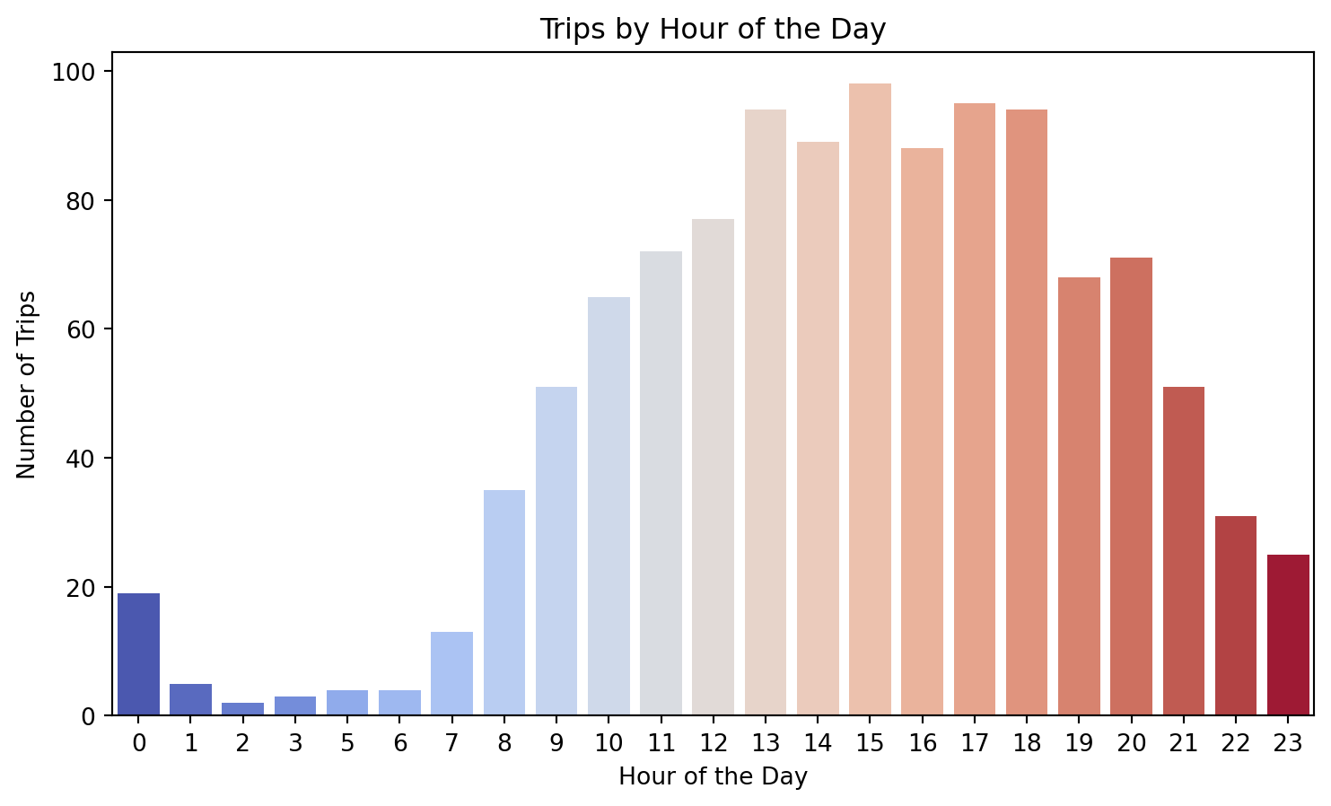

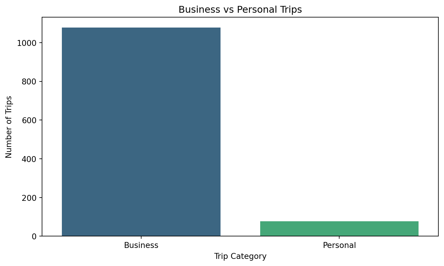
Code for plot of Trip category to number of trips distribution

plt.figure(figsize=(9, 5))
sns.countplot(x=df["category"], hue=df["category"], palette="viridis", legend=False)
plt.xlabel("Trip Category")
plt.ylabel("Number of Trips")
plt.title("Business vs Personal Trips")
plt.show()